44 excel scatter diagram with labels

Add labels to scatter graph - Excel 2007 - MrExcel Message Board Nov 10, 2008. #1. OK, so I have three columns, one is text and is a 'label' the other two are both figures. I want to do a scatter plot of the two data columns against each other - this is simple. However, I now want to add a data label to each point which reflects that of the first column - i.e. I don't simply want the numerical value or ... Creating Scatter Plot with Marker Labels - Microsoft Community Right click any data point and click 'Add data labels and Excel will pick one of the columns you used to create the chart. Right click one of these data labels and click 'Format data labels' and in the context menu that pops up select 'Value from cells' and select the column of names and click OK.

How to rotate axis labels in chart in Excel? - ExtendOffice 1. Go to the chart and right click its axis labels you will rotate, and select the Format Axis from the context menu. 2. In the Format Axis pane in the right, click the Size & Properties button, click the Text direction box, and specify one direction from the drop down list. See screen shot below:

Excel scatter diagram with labels

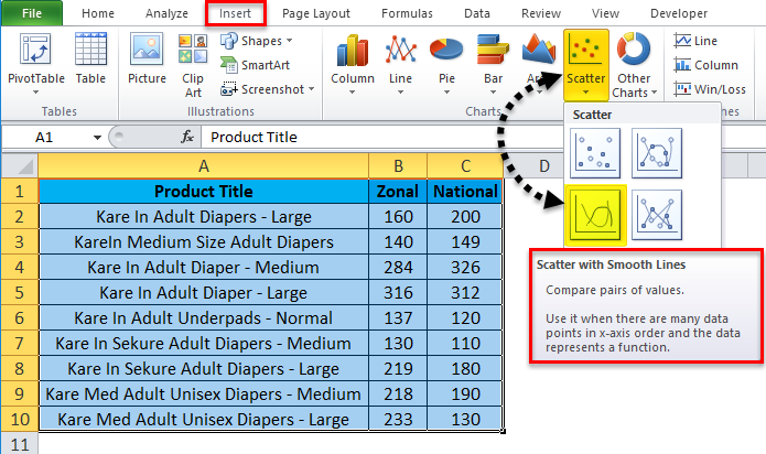
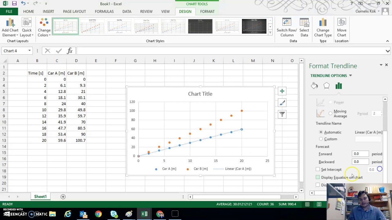
Add Custom Labels to x-y Scatter plot in Excel Step 1: Select the Data, INSERT -> Recommended Charts -> Scatter chart (3 rd chart will be scatter chart) Let the plotted scatter chart be. Step 2: Click the + symbol and add data labels by clicking it as shown below. Step 3: Now we need to add the flavor names to the label. Now right click on the label and click format data labels. Excel scatter chart using text name - Access-Excel.Tips Since Excel allows different chart types to be displayed in one chart, we are going to create a mix of bar chart (column chart) and scatter chart. Scatter chart is used to display the actual data point, while bar chart is to display Grade labels. - Create scatter chart for Range B20:C31 (Series 1) Add vertical line to Excel chart: scatter plot, bar and line graph ... For the main data series, choose the Line chart type. For the Vertical Line data series, pick Scatter with Straight Lines and select the Secondary Axis checkbox next to it. Click OK. Right-click the chart and choose Select Data…. In the Select Data Source dialog box, select the Vertical Line series and click Edit.

Excel scatter diagram with labels. XY Scatter Diagram - Excel Help Forum I saw your axis labels are Y = Consequence and X = Prob but the data source for the chart in your file is Y = Prob and X = Consq, so I changed it in this attached file to be align with axis title. Attached Files Analysis.xlsx‎ (60.2 KB, 6 views) Download Register To Reply 03-21-2022, 12:40 PM #3 MarvinP Forum Guru Join Date 07-23-2010 Location How To Add Axis Labels In Excel [Step-By-Step Tutorial] If you would only like to add a title/label for one axis (horizontal or vertical), click the right arrow beside 'Axis Titles' and select which axis you would like to add a title/label. Editing the Axis Titles After adding the label, you would have to rename them yourself. There are two ways you can go about this: Manually retype the titles How To Create Scatter Chart in Excel? - EDUCBA To apply the scatter chart by using the above figure, follow the below-mentioned steps as follows. Step 1 - First, select the X and Y columns as shown below. Step 2 - Go to the Insert menu and select the Scatter Chart. Step 3 - Click on the down arrow so that we will get the list of scatter chart list which is shown below. Present your data in a scatter chart or a line chart Click the Insert tab, and then click Insert Scatter (X, Y) or Bubble Chart. Click Scatter. Tip: You can rest the mouse on any chart type to see its name. Click the chart area of the chart to display the Design and Format tabs. Click the Design tab, and then click the chart style you want to use. Click the chart title and type the text you want.

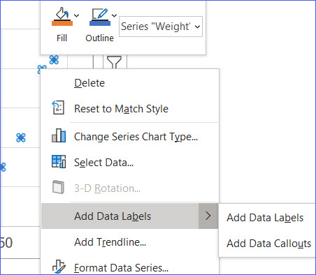
How to Add Labels to Scatterplot Points in Excel - Statology Step 3: Add Labels to Points. Next, click anywhere on the chart until a green plus (+) sign appears in the top right corner. Then click Data Labels, then click More Options…. In the Format Data Labels window that appears on the right of the screen, uncheck the box next to Y Value and check the box next to Value From Cells. How to Create Scatter Plots in Excel (In Easy Steps) To create a scatter plot with straight lines, execute the following steps. 1. Select the range A1:D22. 2. On the Insert tab, in the Charts group, click the Scatter symbol. 3. Click Scatter with Straight Lines. Note: also see the subtype Scatter with Smooth Lines. Note: we added a horizontal and vertical axis title. How to find, highlight and label a data point in Excel scatter plot Select the Data Labels box and choose where to position the label. By default, Excel shows one numeric value for the label, y value in our case. To display both x and y values, right-click the label, click Format Data Labels…, select the X Value and Y value boxes, and set the Separator of your choosing: Label the data point by name How to Make a Scatter Plot in Excel | GoSkills How to make a scatter plot in Excel Let's walk through the steps to make a scatter plot. Step 1: Organize your data Ensure that your data is in the correct format. Since scatter graphs are meant to show how two numeric values are related to each other, they should both be displayed in two separate columns.

How to Create a Scatterplot with Multiple Series in Excel Step 3: Create the Scatterplot. Next, highlight every value in column B. Then, hold Ctrl and highlight every cell in the range E1:H17. Along the top ribbon, click the Insert tab and then click Insert Scatter (X, Y) within the Charts group to produce the following scatterplot: The (X, Y) coordinates for each group are shown, with each group ... Excel Scatter Chart with Labels - Super User Move the button down and out of the way of your data if you have more than a few columns. Paste your data in on top of the film data. Create scatter plots by selecting two column at a time and insert scatter (plot). Clicking on the button, which will add labels. Easy. Excel 2019/365: Scatter Plot with Labels - YouTube How to add labels to the points on a scatter plot. How to Make a Scatter Plot in Excel with Two Sets of Data? To get started with the Scatter Plot in Excel, follow the steps below: Open your Excel desktop application. Open the worksheet and click the Insert button to access the My Apps option. Click the My Apps button and click the See All button to view ChartExpo, among other add-ins.

X-Y Chart (Excel 2010) - Step 2 Construct a Scatter Chart with Labels - YouTube

How to add conditional colouring to Scatterplots in Excel Step 3: Edit the colours. To edit the colours, select the chart -> Format -> Select Series A from the drop down on top left. In the format pane, select the fill and border colours for the marker. Repeat these steps for Series B and Series C. Here is our final scatterplot.

How to Make a Scatter Plot in Excel - BSUPERIOR

Improve your X Y Scatter Chart with custom data labels Select the x y scatter chart. Press Alt+F8 to view a list of macros available. Select "AddDataLabels". Press with left mouse button on "Run" button. Select the custom data labels you want to assign to your chart. Make sure you select as many cells as there are data points in your chart. Press with left mouse button on OK button. Back to top

How to join the points on a scatter plot in Excel - YouTube

How to use a macro to add labels to data points in an xy scatter chart ... In Microsoft Office Excel 2007, follow these steps: Click the Insert tab, click Scatter in the Charts group, and then select a type. On the Design tab, click Move Chart in the Location group, click New sheet , and then click OK. Press ALT+F11 to start the Visual Basic Editor. On the Insert menu, click Module.

Scatter Chart in Excel (Examples) | How To Create Scatter Chart in Excel?

How to Create Scatter Plot In Excel - Career Karma 2. Display the Scatter Chart. Once you have inputted the data, select the desired columns, go to the Insert tab in Excel, select the XY Scatter Chart and choose the first scatter plot option. Now you should have a scatter graph shown in your Excel file. With this done, you need to add a chart title to the scatter plot.

How to Make a Scatter Chart - ExcelNotes

Labeling points in excel scatter diagram - YouTube Showing how to put labels on points of an excel scatter diagram. The video can help familiarize with plotting a scatter diagram, putting trendlines, formatting the chart, x and y axis, use of...

How to Create a Scatter Diagram in Excel - YouTube

excel - How to label scatterplot points by name? - Stack Overflow select a label. When you first select, all labels for the series should get a box around them like the graph above. Select the individual label you are interested in editing. Only the label you have selected should have a box around it like the graph below. On the right hand side, as shown below, Select "TEXT OPTIONS".

How To Create A Scatter Plot In Excel - slideshare

Bubble Chart in Excel (Examples) | How to Create Bubble Chart? Step 7 - Adding data labels to the chart. For that, we have to select all the Bubbles individually. Once you have selected the Bubbles, press right-click and select "Add Data Label". Excel has added the values from life expectancies to these Bubbles, but we need the values GDP for the countries.

Scatter Diagram to Print | 101 Diagrams

Use text as horizontal labels in Excel scatter plot Edit each data label individually, type a = character and click the cell that has the corresponding text. This process can be automated with the free XY Chart Labeler add-in. Excel 2013 and newer has the option to include "Value from cells" in the data label dialog. Format the data labels to your preferences and hide the original x axis labels.

How To Make A Scatter Plot In Excel

How to display text labels in the X-axis of scatter chart in Excel? Display text labels in X-axis of scatter chart Actually, there is no way that can display text labels in the X-axis of scatter chart in Excel, but we can create a line chart and make it look like a scatter chart. 1. Select the data you use, and click Insert > Insert Line & Area Chart > Line with Markers to select a line chart. See screenshot: 2.

Microsoft Excel - Creating a Scatter Plot with trend line and axis labels - YouTube

Scatter Graph - Overlapping Data Labels - Excel Help Forum We are not able to work with or manipulate a picture of one and nobody wants to have to recreate your data from scratch. 1. Make sure that your sample data are REPRESENTATIVE of your real data. The use of unrepresentative data is very frustrating and can lead to long delays in reaching a solution. 2.

Scatter Chart in Microsoft Excel

Excel Charts - Scatter (X Y) Chart - Tutorials Point Step 1 − Arrange the data in columns or rows on the worksheet. Step 2 − Place the x values in one row or column, and then enter the corresponding y values in the adjacent rows or columns. Step 3 − Select the data. Step 4 − On the INSERT tab, in the Charts group, click the Scatter chart icon on the Ribbon.

How to Make Scatter Plots in Microsoft Excel 2007 - Bright Hub

Add vertical line to Excel chart: scatter plot, bar and line graph ... For the main data series, choose the Line chart type. For the Vertical Line data series, pick Scatter with Straight Lines and select the Secondary Axis checkbox next to it. Click OK. Right-click the chart and choose Select Data…. In the Select Data Source dialog box, select the Vertical Line series and click Edit.

Fors: Adding labels to Excel scatter charts

Excel scatter chart using text name - Access-Excel.Tips Since Excel allows different chart types to be displayed in one chart, we are going to create a mix of bar chart (column chart) and scatter chart. Scatter chart is used to display the actual data point, while bar chart is to display Grade labels. - Create scatter chart for Range B20:C31 (Series 1)